Wrapping up the rules

… then jumping into applications

Plan

1. Develop the remaining shortcuts for calculating derivatives
2. Work out more examples
3. Interpretations of the derivative, especially in economics
4. Some applications
5. More SymPy here and there

The shortcuts so far

Let \(c\), \(r\) be constants.

1. \(f(x)=c \Rightarrow f^\prime(x)=0\)
2. \(g(x)=cf(x) \Rightarrow g^\prime(x)=cf^\prime(x)\)
3. (Power rule) \(f(x)=x^r \Rightarrow f^\prime(x)=rx^{r-1}\)
4. (Sum rule) If \(F(x)=f(x)\pm g(x)\), then \[F^\prime(x)=f^\prime(x)\pm g^\prime(x).\]

5. (Product rule) If \(F(x)=f(x)\cdot g(x)\), then \[F^\prime(x)=f(x)g^\prime(x)+g(x)f^\prime(x).\]
6. (Quotient rule) If \(F(x)=\dfrac{f(x)}{g(x)}\), then \[F^\prime(x)=\frac{g(x)f^\prime(x)-f(x)g^\prime(x)}{\left(g(x)\right)^2}.\]
7. \(f(x)=e^x \Rightarrow f^\prime(x)=e^x\)

An argument for the sum rule

• Form the Newton quotient

\[\begin{eqnarray*}\frac{F(x+h)-F(x)}{h}&=&\frac{f(x+h)+g(x+h)-f(x)-g(x)}{h} \\ &=& \frac{f(x+h)-f(x)}{h} + \frac{g(x+h)-g(x)}{h}\end{eqnarray*}\]

• Let \(h\to 0\). What do you notice?

An argument for the product rule

• Think of a rectangle with base \(f(x)\) and height \(g(x)\). What is the area of this rectangle?
• Imagine a change from \(x\) to \(x+h\).
• What happens to the original rectangle and its area?
• Let \(h\to 0\). What do you notice?

Shortcut 08: The Chain Rule

1. We had difficulty working with the derivative of \((t^2+4)^{-1}\).
2. We could use the quotient rule here. But it can be a bit too much.
3. Observe that \((t^2+4)^{-1}\) has the form of a power, but we cannot apply the power rule directly.

4. Observe that if we let \(y=f(x)=x^{-1}\) and \(x=g(t)=t^2+4\), then the composition of \(f\) with \(g\) is \[y=f(g(t))=(t^2+4)^{-1}.\]
5. In other words, \(y\) is a function of \(x\) and \(x\) is a function of \(t\). Thus, a “chain” is formed.
6. What happens when \(t=a\) changes to \(t=a+h\)? \(g(a)\) changes to \(g(a+h)\).
7. But that means \(f(g(a))\) changes to \(f(g(a+h))\).

9. Suppose \(k=g(a+h)-g(a)\neq 0\). Observe that \[\begin{eqnarray*} && \frac{f(g(a+h))-f(g(a)}{h} \\ &=& \frac{f(g(a+h))-f(g(a))}{g(a+h)-g(a)}\times\frac{g(a+h)-g(a)}{h} \\ &=& \frac{f(g(a)+k)-f(g(a))}{k}\times\frac{g(a+h)-g(a)}{h}\end{eqnarray*}\]

10. What happens when \(h\to 0\)?

11. As \(h\to 0\), we also have \(k\to 0\).

12. Roughly speaking, we have \[\begin{eqnarray*} && \lim_{h\to 0} \frac{f(g(a+h))-f(g(a))}{h} \\ &=& \lim_{h\to 0}\frac{f(g(a+h))-f(g(a))}{g(a+h)-g(a)}\times\lim_{h\to 0}\frac{g(a+h)-g(a)}{h} \\ &=& \lim_{k\to 0}\frac{f(g(a)+k)-f(g(a))}{k}\times\lim_{h\to 0}\frac{g(a+h)-g(a)}{h} \\ &=& f^\prime (g(a)) g^\prime(a)\end{eqnarray*}\]

Comments about the chain rule

1. The argument I showed is not very complete, but gives a rough idea to understand the shortcut.
2. The chain rule is as follows: Let \(F(t)=f(g(t))\) be a composition of \(f\) with \(g\). If \(g^\prime(t)\) is well-defined and \(f^\prime(g(t))\) is well-defined, then \[F^\prime(t) = f^\prime(g(t))g^\prime(t)\]
3. The composition of \(f\) with \(g\) is in general different from the composition of \(g\) with \(f\).

Examples for the chain rule

1. \(F(t)=(t^2+4)^{-1}\)
2. \(h(x)=(x^3+x^2)^{50}\)
3. \(f(x)=\sqrt{\dfrac{x-1}{x+3}}\)
4. \(g(x)=\sqrt{3x+\sqrt{x}}\)
5. \(h(t)=e^{\sqrt{t}}\)
6. \(f(z)=\left(3e^{z^3}-z^3\right)^{1/3}\)

Taking stock

1. So far, we have a lot of shortcuts and they become the building blocks which enable you to calculate derivatives.
2. Of course, SymPy is available to you for verification.
3. But the “meatier” part of the approach so far was to build the rules you are going to use. From there, you can build even further, as you will see in subsequent applications.
4. We now move on to an alternative interpretation of derivatives, beyond being slopes of curves.

Rates of change

1. We already dipped our toes into the average rate of change interpretation of the Newton quotient.
2. When \(h\to 0\) in the Newton quotient, we now have the instantaneous rate of change.
3. Therefore, \(f^\prime(a)\) is the instantaneous rate of change at \(a\).
4. The relative rate of change at \(a\) is \(\dfrac{f^\prime(a)}{f(a)}\).

Concepts in economics framed in terms of derivatives

1. Capital stock as a function of time: \(K(t)\)

   • Change in the level or investment: \(K(t+h)-K(t)\)
   • Average rate of change: \(\dfrac{K(t+h)-K(t)}{h}\)
   • Investment rate: \(K^\prime(t)\)
   • Growth rate in capital stock: \(\dfrac{K^\prime(t)}{K(t)}\)

2. Costs as a function of units produced: \(C(q)\)

   • Change in the costs: \(C(q+h)-C(q)\)
   • Average rate of change: \(\dfrac{C(q+h)-C(q)}{h}\)
   • Marginal cost: \(C^\prime(q)\)
   • Growth rate in costs: \(\dfrac{C^\prime(q)}{C(q)}\)

3. Revenues as a function of units produced: \(R(q)\)

   • Change in the revenues: \(R(q+h)-R(q)\)
   • Average rate of change: \(\dfrac{R(q+h)-R(q)}{h}\)
   • Marginal revenue: \(R^\prime(q)\)
   • Growth rate in revenues: \(\dfrac{R^\prime(q)}{R(q)}\)

4. There are many other similar framings which you will encounter if you study economics further.

5. The study of certain types of ratios is of interest in economics. For example, the real wage \(w(t)\) as a function of time is the ratio of nominal wages \(W(t)\) to the price index \(P(t)\).

6. The growth rate of real wages over time is \[\frac{w^\prime(t)}{w(t)}=\frac{W^\prime(t)}{W(t)}-\frac{P^\prime(t)}{P(t)}\] The last term is called the inflation rate.

7. Another type of ratio of interest in economics involve ratios of relative changes or elasticities.

8. A very important elasticity used in economics is the price elasticity of demand. This is the ratio of the relative change in quantity demanded and the relative change in price.

9. To make things more concrete, let \(q(p)\) be the quantity demanded as a function of price \(p\).

9. Suppose prices change from \(p\) to \(p+h\). The relative change in price is \[\frac{(p+h)-p}{p}=\dfrac{h}{p}\]

10. The relative change in quantity demanded as a result of a change in price is \[\frac{q(p+h)-q(p)}{q(p)}\]

11. By definition, the price elasticity of demand is the ratio of the relative change in quantity demanded and the relative change in price:

\[\frac{\dfrac{q(p+h)-q(p)}{q(p)}}{\dfrac{h}{p}}=\frac{q(p+h)-q(p)}{h}\times \frac{p}{q(p)}\]

12. Notice the presence of a Newton quotient! Let \(h\to 0\). Then, the price elasticity of demand could be expressed in terms of derivatives and relative rates of change: \[q^\prime(p)\frac{p}{q(p)}=p\frac{q^\prime(p)}{q(p)}\]

13. In more general terms, the elasticity of \(f\) with respect to \(x\) is given by \[\mathsf{el}_x f(x)= x\frac{f^\prime (x)}{f(x)}\]

Moving on

1. Many concepts in economics could be framed in terms of derivatives.

2. We will have a chance to explore the implications of using these derivatives:

   • How are revenues affected by demand conditions?
   • When should a firm increase or decrease production of a good?
   • How does a monopoly charge for a good?

3. But we need to dig deeper.

Application 01: An algorithm to solve difficult equations by hand or through a spreadsheet

1. You may find it easy to solve for \(x\) for the following equations:

   1. \(3x+2=0\)
   2. \(4x^2-3x-1=0\)

2. But what if you are asked to solve for \(x\) in \[x^6 +3x^2-2x-1=0?\] How do you even start?

3. For now, let \(f(x)=x^6 +3x^2-2x-1\).

4. Don’t aim for getting an answer right away. Instead, start with a guess first (whether good or bad).

5. We are going to cheat a bit to have a guess, but this is more for you to see how to develop an algorithm.

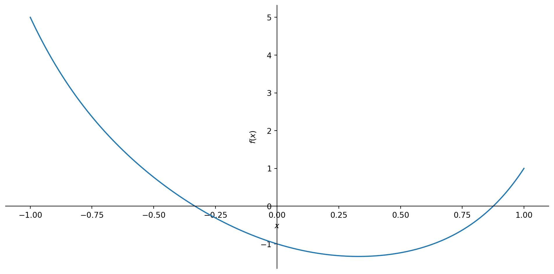
6. Sketch the graph of \(f\) first.

7. Let us start with \(x=-0.5\). Draw the line tangent to \(f\) at \(x=-0.5\).

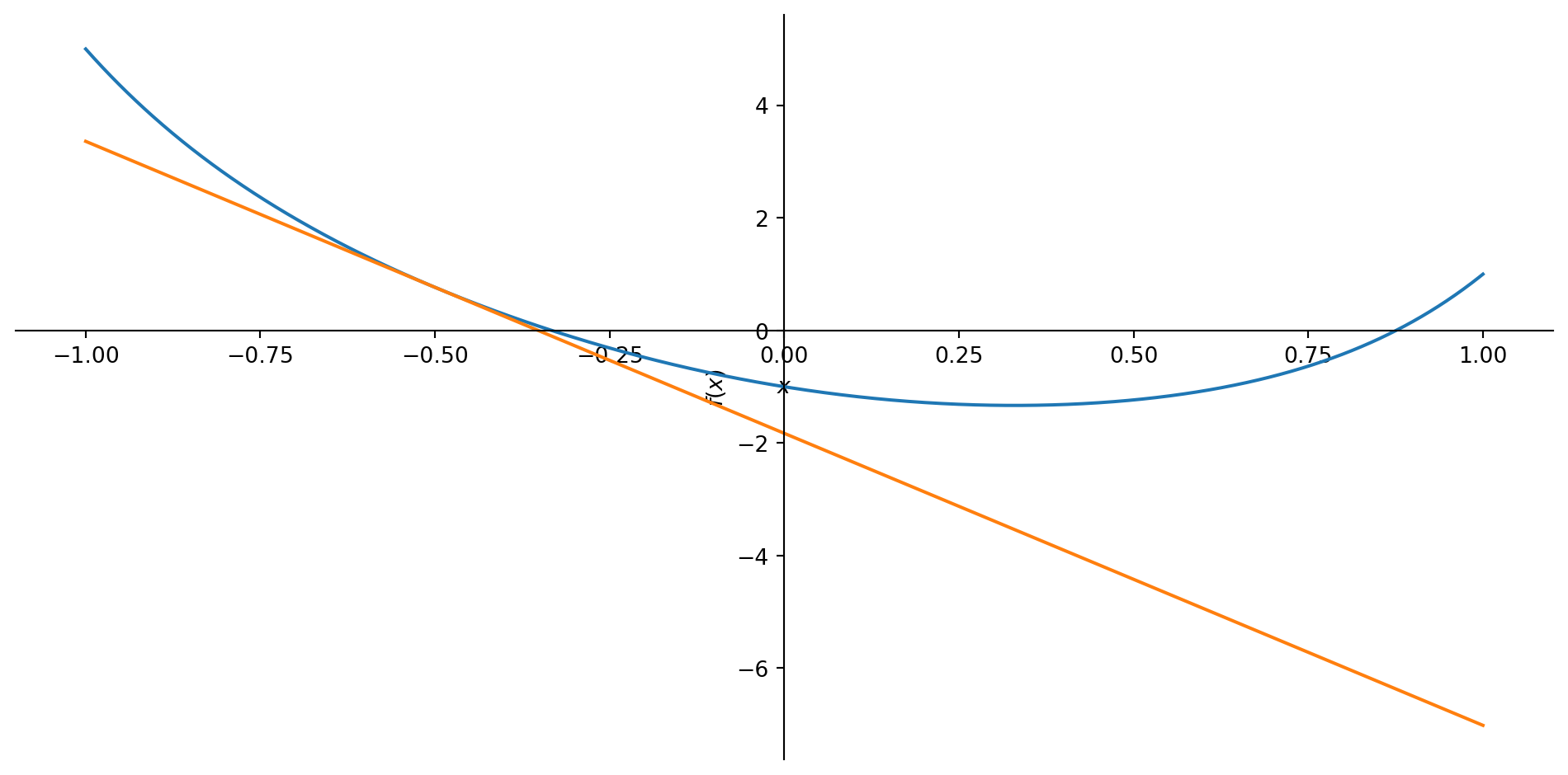
8. Let us zoom in closer.

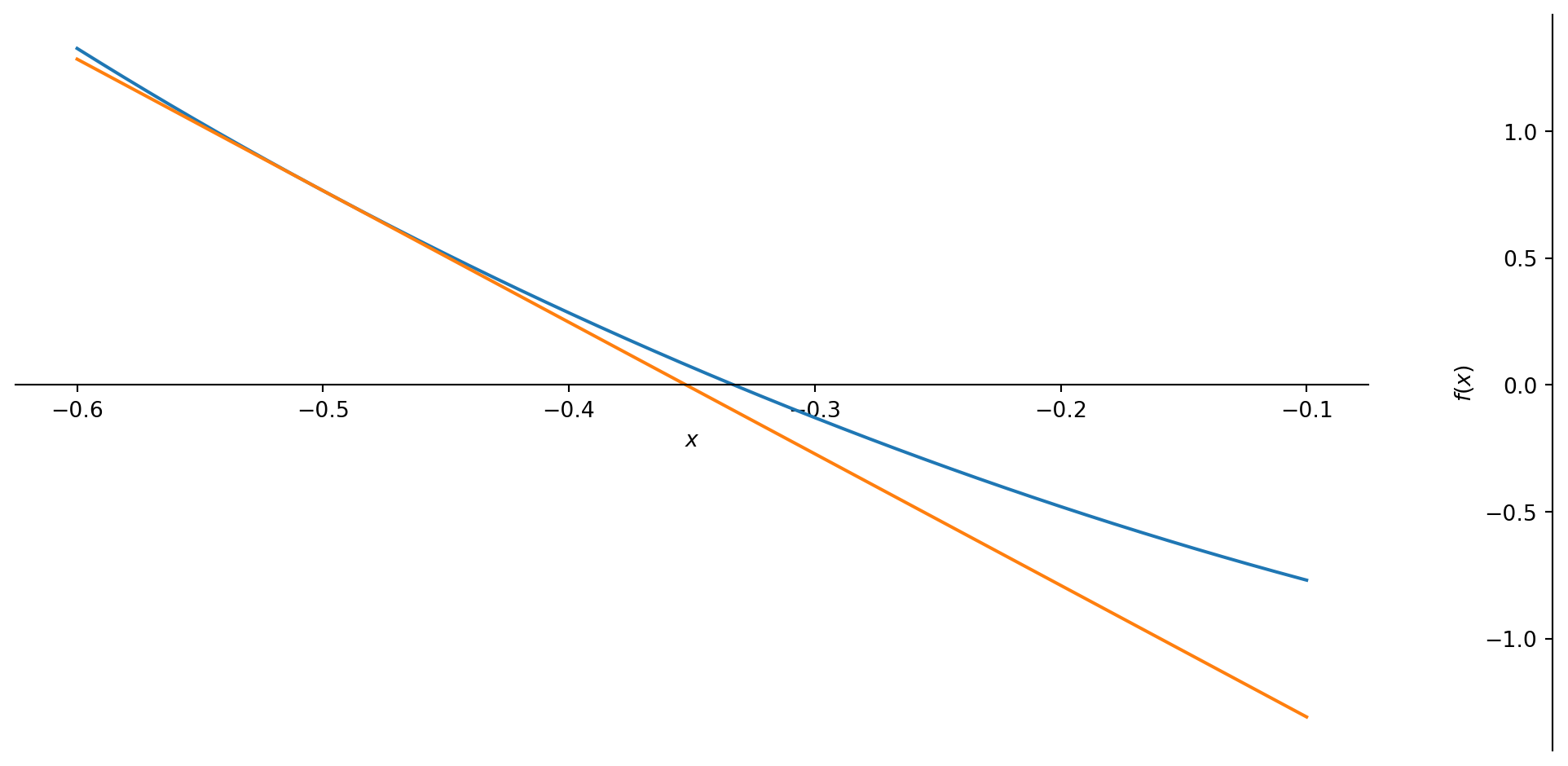
9. Notice that we now have a better guess than when we started at \(x=-0.5\).

10. The better guess is the intersection of the orange line and the horizontal axis crossing the origin.

11. How do we get this new guess? Call the old guess \(x_0\). All we did was to get the equation of the line tangent to \(f\) at \(x=x_0\):

\[P_1(x)=f(x_0)+f^\prime(x_0)(x-x_0)\]

12. The horizontal line crossing the origin is really \(P_1(x)=0\), so the corresponding value of \(x\) when the orange line crosses \(P_1(x)=0\) is \[\begin{eqnarray*}0 &=& f(x_0)+f^\prime(x_0)(x-x_0) \\ -f(x_0) &=& f^\prime(x_0)(x-x_0) \\ -\frac{f(x_0)}{f^\prime(x_0)} &=& x-x_0 \\ x_0-\frac{f(x_0)}{f^\prime(x_0)} &=& x\end{eqnarray*}\]

13. We now have a new guess! Visually it looks like a good guess. Specifically, we have a new guess equal to \[x=x_0-\frac{f(x_0)}{f^\prime(x_0)}\]

14. Repeat the process. Draw the line tangent to \(f\) at your new guess.

15. Zoom in closer.

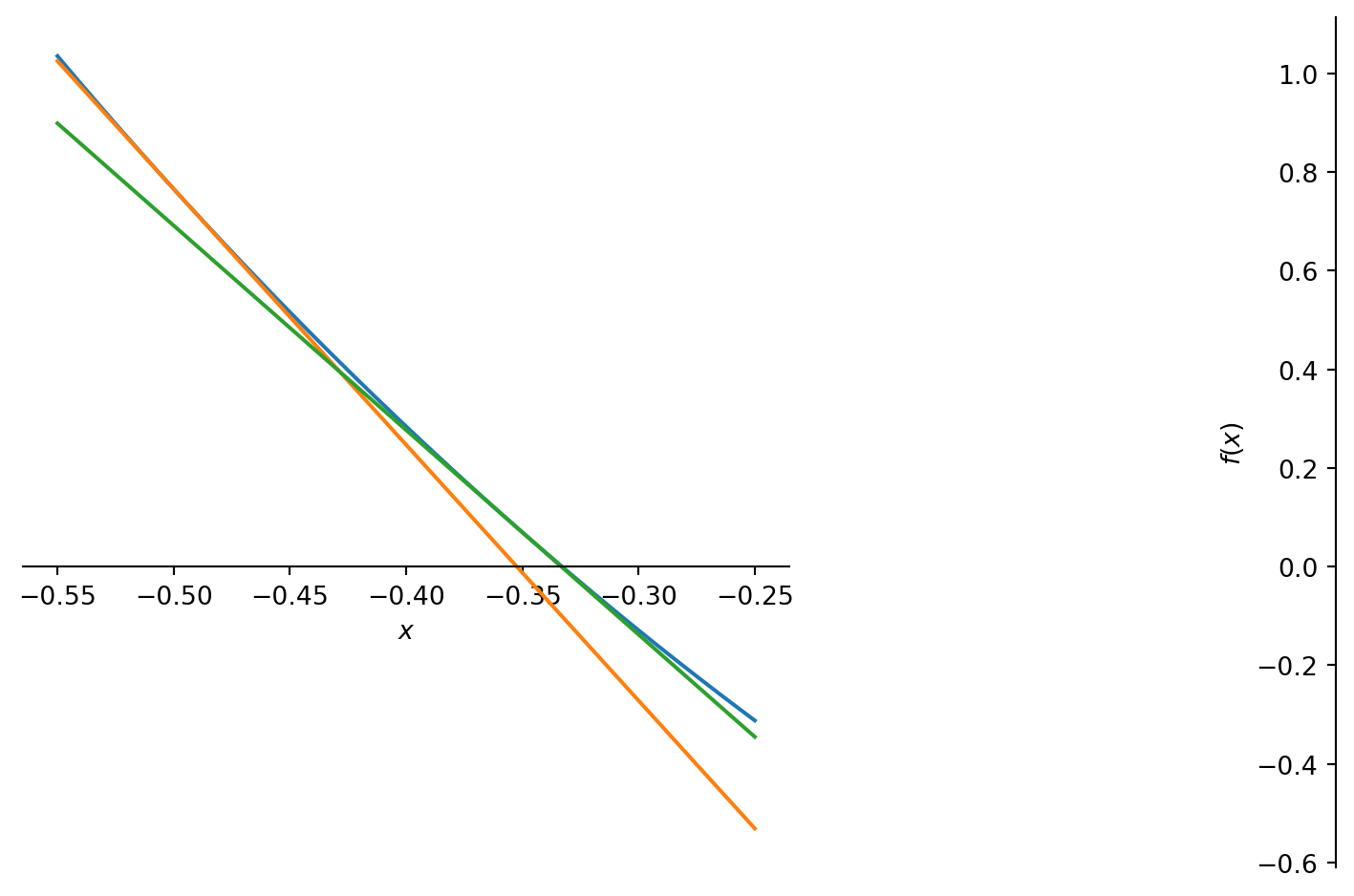
16. Zoom in even closer.

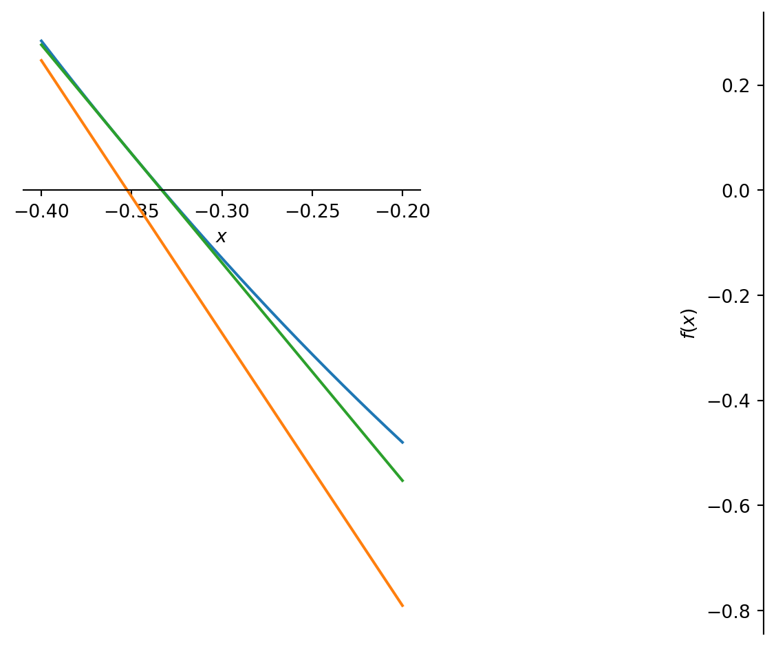
16. Seems like we are getting very near an \(x\) which will solve \(x^6+3x^2-2x-1=0\).

17. We could repeat finding the process of getting another new guess, but it would seem that we are near enough.

18. Congratulations! We have developed an algorithm which enables us to solve for \(x\) in difficult equations. This algorithm is called Newton’s method.

19. SymPy can look for solutions in the following way:

from sympy import *
x = symbols('x', real = True)
nsolve(x**6+3*x**2-2*x-1, x, (-0.4, -0.2))

\(\displaystyle -0.332992409726606\)

Algorithm for Newton’s method

Use case: Solving for \(x\) in \(f(x)=0\) in some specified interval \([a,b]\).

1. Start with an initial guess \(x_0\in[a,b]\). Start with \(i=1\).
2. Get the next guess \(x_i\) as \[x_i=x_{i-1}-\frac{f(x_{i-1})}{f^\prime(x_{i-1})}\]
3. Increase \(i\) by 1 and repeat step 2.
4. Have a rule as to when to stop.

Application 02: Implicit functions

1. All the functions you have encountered so far are of the form \(y=f(x)\) where \(y\) is written explicitly as a function of \(x\).

2. What happens if this is not the case?

3. Consider the case \(x=e^y\), where \(y=f(x)\). What is \(f^\prime(x)\)?

   • One approach is to solve for \(y\) in terms of \(x\), then calculate \(f^\prime(x)\) directly.
   • Another approach is to indirectly recover \(f^\prime(x)\) from \(x=e^y\).

We use the second approach. Start with \(x=e^y\).

1. Take derivatives of both sides of the equation with respect to \(x\).
2. We get \(1 = e^y f^\prime(x)\). How did we get this?
3. Solve for \(f^\prime(x)\) and write everything in terms of \(x\) if possible:

\[\begin{eqnarray*}1 = e^y f^\prime(x) \Rightarrow \frac{1}{e^y}=f^\prime(x) \\ \Rightarrow \frac{1}{x}=f^\prime (x)\end{eqnarray*}\]

We could obtain the result in SymPy:

from sympy import *
x, y = symbols('x y', real = True)
idiff(x-exp(y), y , x)

\(\displaystyle e^{- y}\)

But this is really \(1/x\) after some further processing.

The approach you have just witnessed is called implicit differentiation.

Congratulations! We have developed a new rule for derivatives.

• In \(x=e^y\), we call \(y\) the natural logarithm of \(x\).
• We write \(y = \ln x\).
• So if \(f(x)=\ln x\), then \(f^\prime(x)=\dfrac{1}{x}\).

Another example of an implicit function

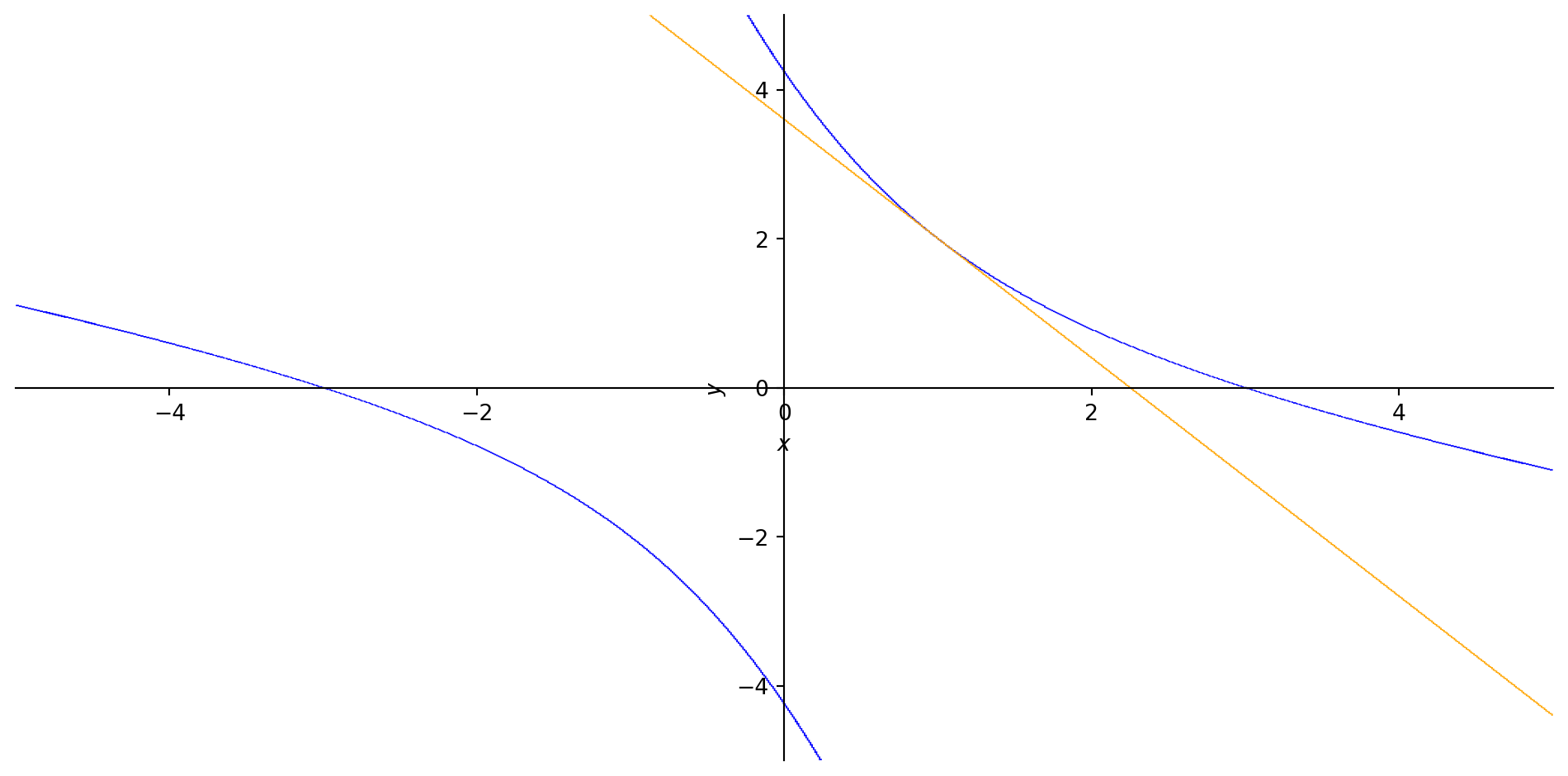
Suppose \(x\) and \(y\) are functionally related by the following equation: \[2x^2+6xy+y^2 =18\]

Find the equation of the line tangent to the curve at \((x,y)=(1,2)\).

We can try using SymPy.

from sympy import *
x, y = symbols('x y', real = True)
idiff(2*x**2 + 6*x*y + y**2 - 18, y , x)

\(\displaystyle - \frac{2 x + 3 y}{3 x + y}\)

So, the slope will be

from sympy import *
x, y = symbols('x y', real = True)
idiff(2*x**2 + 6*x*y + y**2 - 18, y , x).subs({x:1, y:2})

\(\displaystyle - \frac{8}{5}\)

The equation of the line tangent to the given curve is now \[P_1(x)=2-\frac{8}{5}(x-1)=\frac{18}{5}-\frac{8}{5}x\]

Looking forward

• Surely, there has to be shortcuts in calculating the derivative. (Completed, at least those regularly used in economics)
• How do we interpret these derivatives? We actually already started. (Almost completed, moving on to shapes later)
• We may have to dig in a bit into the concept of getting “closer and closer”.

• What if we have even more complicated functions? (Completed, but moving on to functions of more than one variable soon)
• Where is the economics? (Partially completed, will dig further into other applications of differential calculus to economics)