\(\displaystyle - \frac{e^{\frac{1}{x}}}{x^{2}}\)
More applications of the derivative
Plan
- The different notations for a derivative
- Derivative of a derivative? What’s the point?
- Other information contained in derivatives
- Polynomial approximations
- Economic applications
The different notations for the derivative
If \(y=f(x)\), then the derivative with respect to \(x\) could be written in various ways:
- Using the \(\dfrac{d}{dx}\) notation: \(\dfrac{d}{dx} f(x),\ \dfrac{d}{dx}y,\ \dfrac{df(x)}{dx},\ \dfrac{dy}{dx}\)
- Using the prime notation: \(f^\prime(x), f^\prime, y^\prime\)
Some of these notations may be clearer than others. Use the clearer one in your situation.
Higher-order derivatives
- Let \(f(x)\) be some function. The derivative \(f^\prime(x)\) is also a function.
- It is conceivable to think about the derivative of a derivative.
- By definition of the derivative of \(f\), we write \[f^\prime(x)=\lim_{h\to 0}\frac{f(x+h)-f(x)}{h}.\]
- What if we replace \(f\) with \(f^\prime\)? Consider \[\frac{f^\prime(x+h)-f^\prime(x)}{h}.\]
- Letting \(h\to 0\), we obtain the derivative of \(f^\prime(x)\) with respect to \(x\).
- The resulting derivative is called the second derivative of \(f(x)\). This is sometimes written as \(f^{\prime\prime}(x)\).
Perhaps unsurprisingly, \(f^\prime(x)\) is called the first derivative of \(f(x)\).
There are other higher-order derivatives like the third derivative, fourth derivative, and so on. The notation would be \(f^{(3)}(x)\), \(f^{(4)}(x)\), respectively.
It is relatively rare to encounter third and other higher-order derivatives, as first and second derivatives are used more frequently.
Working out some examples
- Find the first six derivatives of \(f(x)=x^5-3x^4+2\).
- Find the second derivative of \(g(x)=e^{1/x}\).
- Let \(f(x)\) and \(g(x)\) be some given functions. Find the second derivative of \(\dfrac{f(x)}{g(x)}\).
- Find the second derivative of \(h(x)=(\ln x+3x^2)^2\).
How do you compute higher-order derivatives in SymPy?
Unspecified functions in SymPy
\(\displaystyle \frac{d}{d x} f{\left(x \right)}\)
from sympy import *
x = symbols('x', real = True)
f = Function('f')
g = Function('g')
diff(f(x)/g(x), x, 2).simplify()
\(\displaystyle \frac{- \left(g{\left(x \right)} \frac{d^{2}}{d x^{2}} g{\left(x \right)} - 2 \left(\frac{d}{d x} g{\left(x \right)}\right)^{2}\right) f{\left(x \right)} + g^{2}{\left(x \right)} \frac{d^{2}}{d x^{2}} f{\left(x \right)} - 2 g{\left(x \right)} \frac{d}{d x} f{\left(x \right)} \frac{d}{d x} g{\left(x \right)}}{g^{3}{\left(x \right)}}\)
\(f\), \(f^\prime\), and \(f^{\prime\prime}\)
Consider \(f(x)=x\). What are the first two derivatives? In a picture:
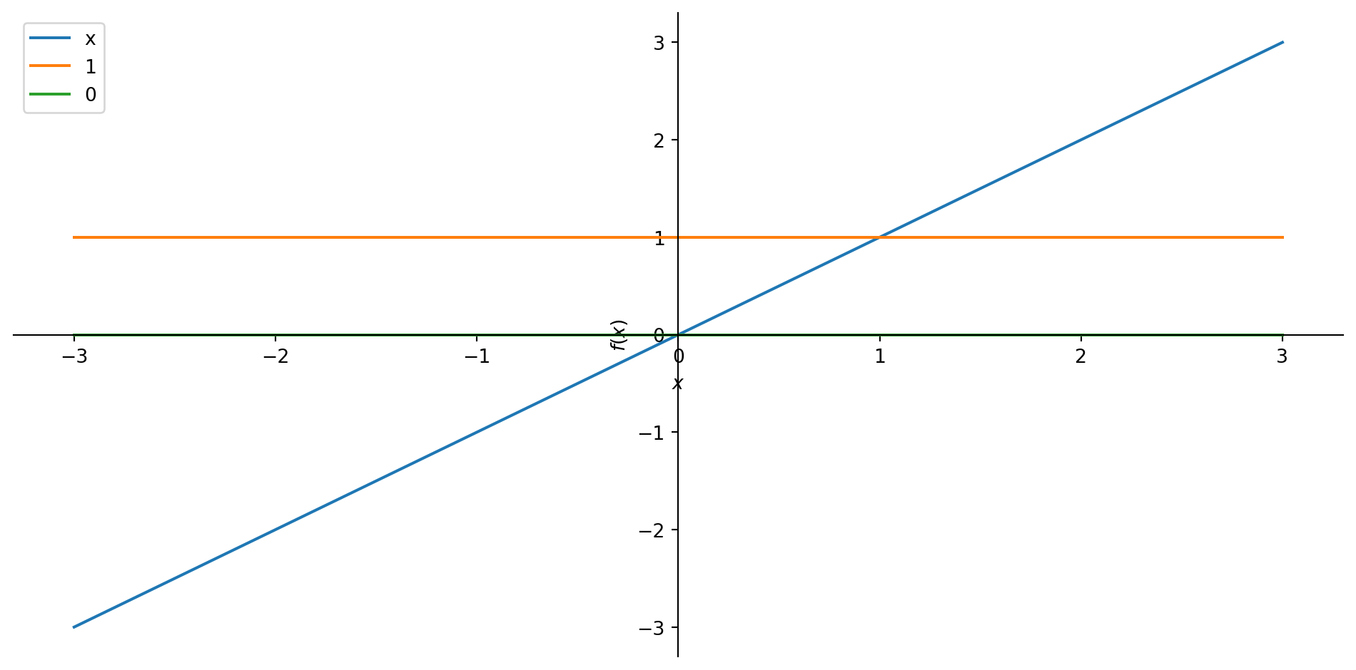
\(f\), \(f^\prime\), and \(f^{\prime\prime}\)
Consider \(f(x)=x^2\). What are the first two derivatives? In a picture:
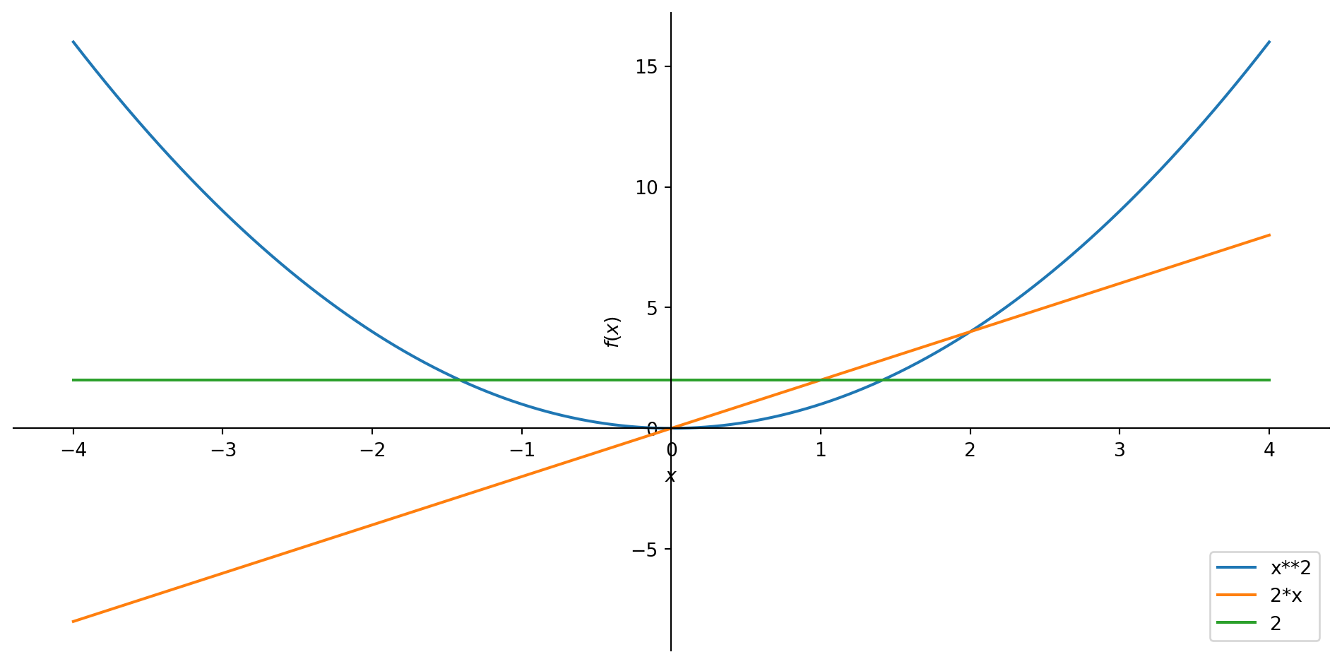
\(f\), \(f^\prime\), and \(f^{\prime\prime}\)
Consider \(f(x)=x^3\). What are the first two derivatives? In a picture:
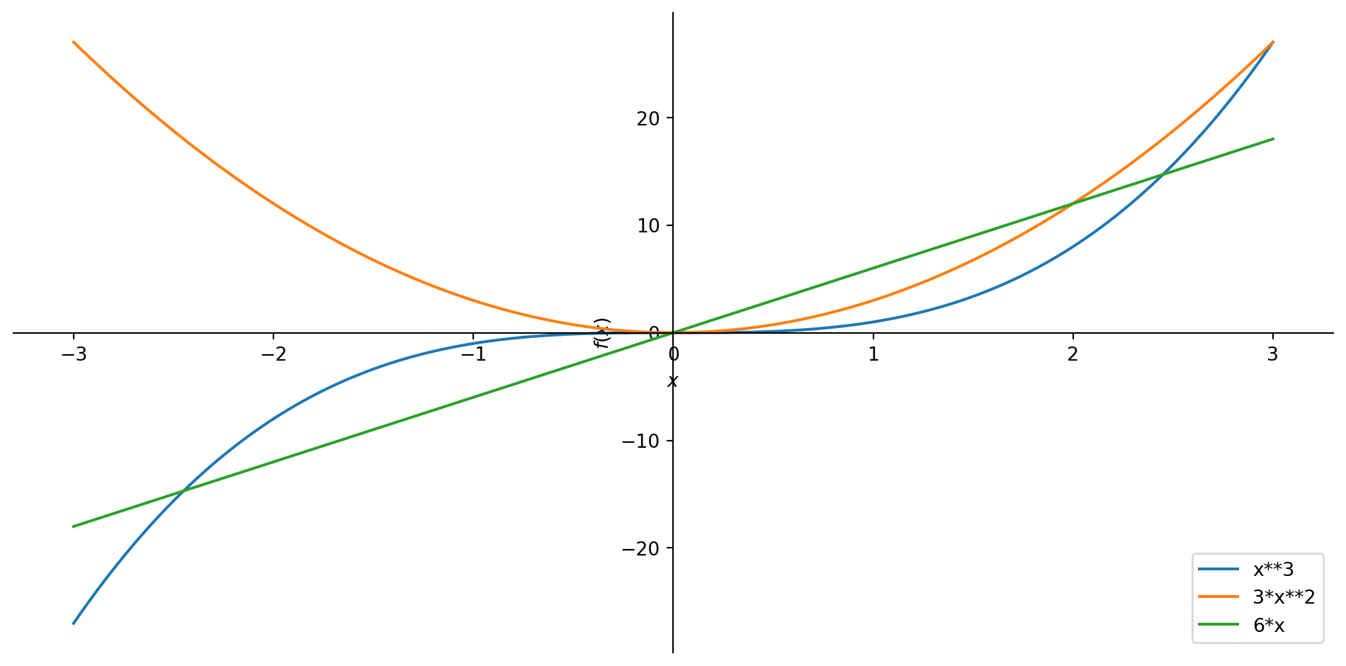
\(f\), \(f^\prime\), and \(f^{\prime\prime}\)
Consider \(f(x)=e^x\). What are the first two derivatives? In a picture:
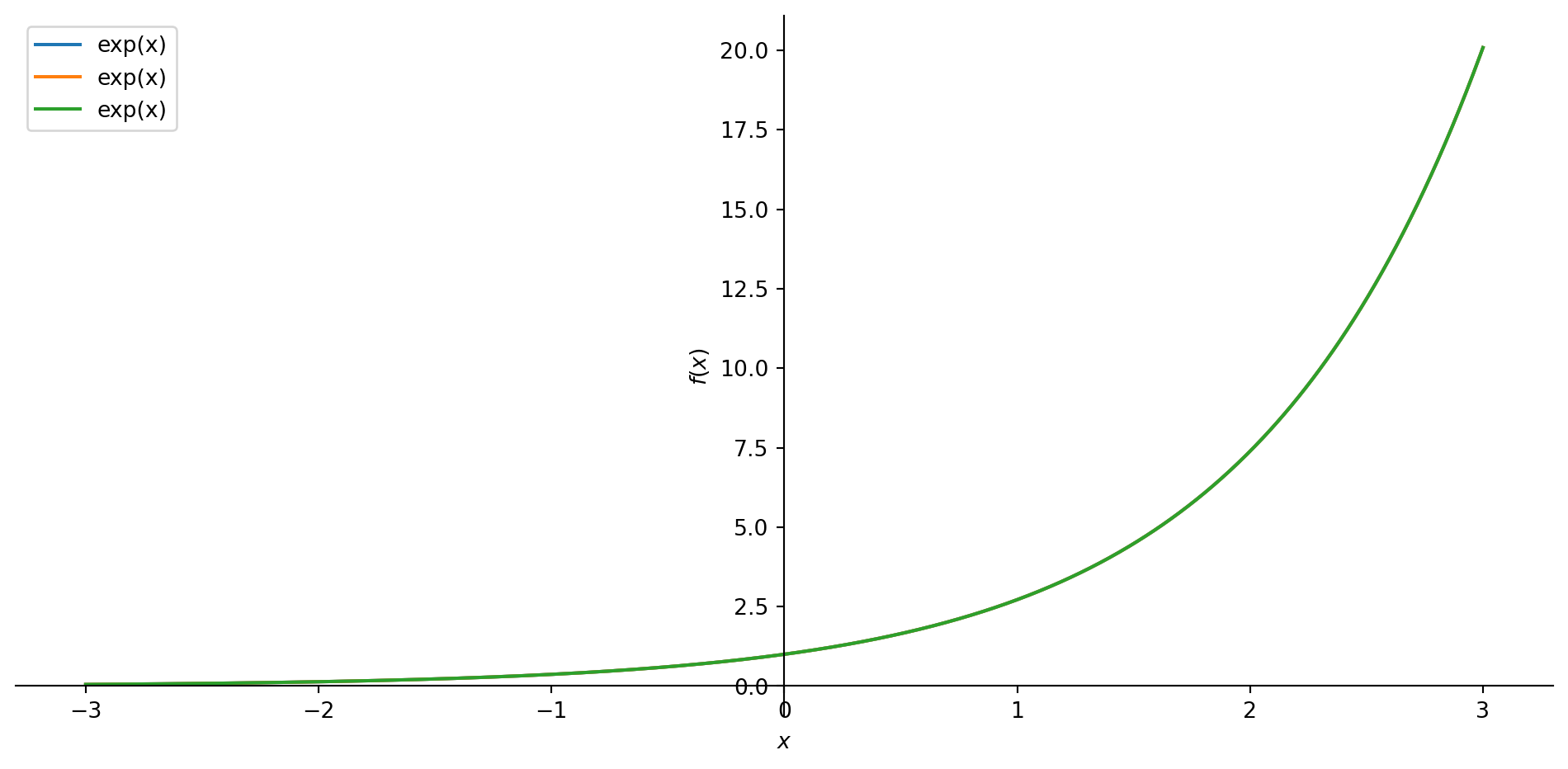
\(f\), \(f^\prime\), and \(f^{\prime\prime}\)
Consider \(f(x)=\ln x\). What are the first two derivatives? In a picture:
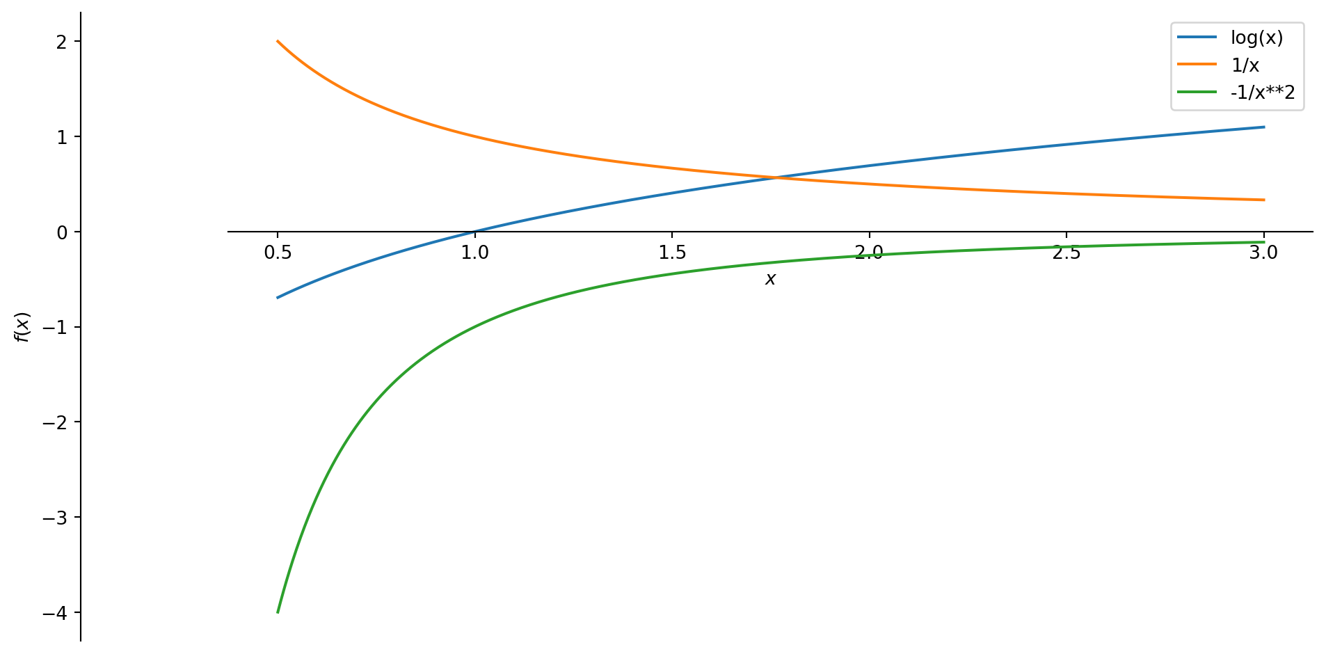
\(f\), \(f^\prime\), and \(f^{\prime\prime}\)
Consider \(c(t)=t/(t^2+4)\). What are the first two derivatives? In a picture:
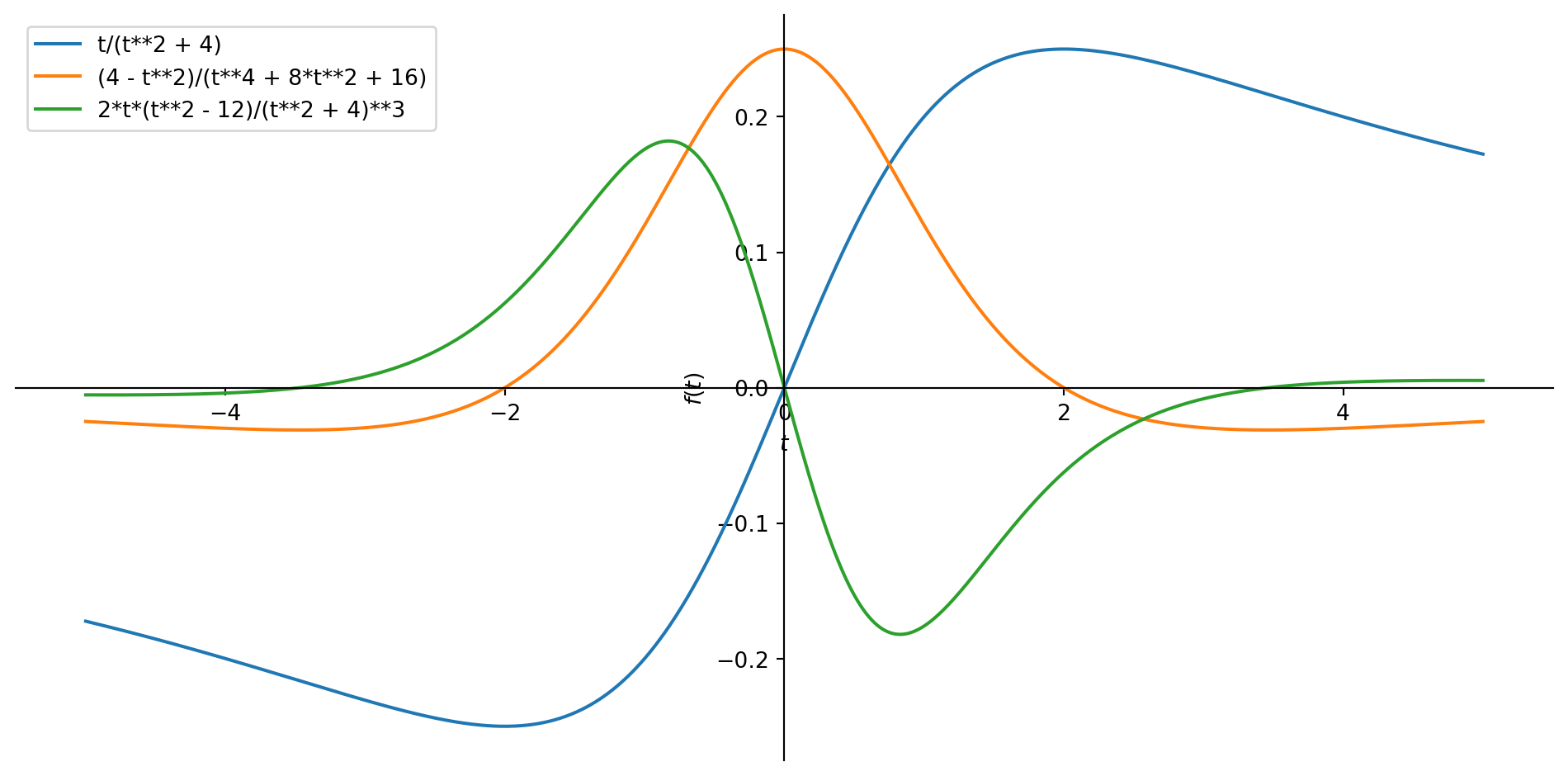
What information do \(f\), \(f^\prime\), and \(f^{\prime\prime}\) contain?
The previous pictures should give you a sense that \(f\), \(f^\prime\), and \(f^{\prime\prime}\) have some important pieces of information which allow you to recover one from the other.
Why is this an important step to learn?
- Most functions considered in economics are incompletely specified.
- Most of the time the signs of the derivatives are available.
- \(f^\prime(x)\geq 0\) over some range is equivalent to saying \(f(x)\) is increasing over that range.
- \(f^\prime(x)\leq 0\) over some range is equivalent to saying \(f(x)\) is decreasing over that range.
- \(f^{\prime\prime}(x)\geq 0\) over some range is equivalent to saying \(f^\prime(x)\) is increasing over that range.
- \(f^{\prime\prime}(x)\leq 0\) over some range is equivalent to saying \(f^\prime(x)\) is decreasing over that range.
Application 03: Approximations
You have already encountered a linear approximation to \(f\) at some point \(x=x_0\). This is nothing but the equation of the tangent line: \[P_1(x)=f(x_0)+f^\prime(x_0)(x-x_0).\]
- Observe that \(P_1(x_0)=f(x_0)\): \(f\) and its approximation match at \(x=x_0\).
- Observe that \(P_1^\prime(x_0)=f^\prime(x_0)\): \(f\) and its approximation have derivatives at \(x=x_0\) that match.
Now, consider improving the approximation to include a quadratic term: \[P_2(x)=P_1(x)+c_2 (x-x_0)^2.\] The problem is that \(c_2\) is unknown.
- You still want \(f\) and the improved approximation to match at \(x=x_0\).
- You still want \(f\) and the improved approximation to have first derivatives that match at \(x=x_0\).
- These imply that we want \(P_2(x_0)=f(x_0)\) and \(P_2^\prime(x_0)=f^\prime(x_0)\).
How should you determine \(c_2\) in \[P_2(x)=P_1(x)+c_2 (x-x_0)^2?\]
- You want \(P_2(x_0)=f(x_0)\) and \(P_2^\prime(x_0)=f^\prime(x_0)\).
- \(P_2(x_0)=f(x_0)\) is satisfied by default.
- \(P_2^\prime(x)=f^\prime(x_0)+2c_2(x-x_0)\), so \(P_2^\prime(x_0)=f^\prime(x_0)\) is also satisfied by default.
- We need an additional restriction to help us obtain \(c_2\).
Why not let the second derivatives of \(f\) and its approximation match?
- Observe that \(P_2^{\prime\prime}(x)=2c_2\).
- Since we want to match the second derivatives of \(P_2(x)\) and \(f(x)\), we want \[2c_2=f^{\prime\prime}(x_0)\Rightarrow c_2=\frac{f^{\prime\prime}(x_0)}{2}.\]
Therefore, the quadratic approximation of \(f\) at \(x=x_0\) is \[P_2(x)=f(x_0)+f^\prime(x_0)(x-x_0)+\frac{f^{\prime\prime}(x_0)}{2}(x-x_0)^2.\]
Sometimes, this is called the second-order Taylor expansion at \(x=x_0\).
Recall our \(c(t)=\dfrac{t}{t^2+4}\) example.
It is possible to consider the third-order or even higher-order approximations, but we do not cover them here.
Application 04: When should a firm increase or decrease production of a good?
Let \(R(q)\) and \(C(q)\) be the revenue and cost functions of a firm producing \(q\) units.
If a firm is interested in profits, it will be interested in \(\pi(q)=R(q)-C(q)\).
Suppose a firm is producing at level \(q=q_1\). Then profits are equal to \(\pi(q_1)\).
Let us say the firm want to change production to \(q_2=q_1+h\), where \(h\neq 0\). Then, profits at the new level would be \(\pi(q_2)=\pi(q_1+h)\). Is the change in production a good idea?
One way to measure this is to look at how profit changed for every change in quantity produced – that is none other than the Newton quotient! Thus, we have \[\frac{\pi(q_2)-\pi(q_1)}{q_2-q_1}=\frac{\pi(q_1+h)-\pi(q_1)}{h}.\]
If \[\frac{\pi(q_1+h)-\pi(q_1)}{h}\geq 0\] for \(h\neq 0\), then
- Increasing production from \(q_1\) to \(q_1+h\) leads to an increase in profits.
- Decreasing production from \(q_1\) to \(q_1+h\) leads to a decrease in profits.
- Therefore, it makes sense to increase production.
If \[\frac{\pi(q_1+h)-\pi(q_1)}{h}\leq 0\] for \(h\neq 0\), then
- Increasing production from \(q_1\) to \(q_1+h\) leads to an decrease in profits.
- Decreasing production from \(q_1\) to \(q_1+h\) leads to a increase in profits.
- Therefore, it makes sense to decrease production.
If we frame what you saw earlier in terms of derivatives, we
- Increase production from \(q_1\) whenever \(\pi^\prime(q_1)\geq 0\).
- Decrease production from \(q_1\) whenever \(\pi^\prime(q_1)\leq 0\).
So, when do you know that you should stop adjusting production? When \(q_1\) is the level at which \(\pi^\prime(q_1)=0\).
We can frame everything in terms of marginal revenues and marginal costs:
- Increase production from \(q_1\) whenever \(R^\prime(q_1)\geq C^\prime(q_1)\).
- Decrease production from \(q_1\) whenever \(R^\prime(q_1)\leq C^\prime(q_1)\).
- Stop adjusting production at \(q_1\) whenever \(R^\prime(q_1)= C^\prime(q_1)\).
This is a key economic idea that actions are examined in terms of marginal benefits and marginal costs!
Application 05: How are revenues affected by demand conditions?
- Suppose a firm faces a demand function \(q(p)\).
- The revenues earned by the firm would be price times the quantity sold. Therefore, revenues would be \(p\times q(p)\).
- How do revenues change when prices change? This is just \[\frac{d}{dp}\left[p\times q(p)\right]=pq^\prime(p)+q(p)\]
- We can rewrite the result in terms of the price elasticity of demand: \[\begin{eqnarray*}\frac{d}{dp}\left[p\times q(p)\right] &=& pq^\prime(p)+q(p) \\ &=& q(p)\left[\frac{pq^\prime(p)}{q(p)}+1\right] \\ &=& q(p)\left[1+\mathsf{el}_p q(p)\right]\end{eqnarray*}\]
Therefore, we have some cases to consider:
- If \(\mathsf{el}_p q(p)=-1\), then a small price change has no effect on revenue.
- If \(-1<\mathsf{el}_p q(p)\leq 0\), then a small increase in price has a positive effect on revenue.
- If \(\mathsf{el}_p q(p)<-1\), then a small increase in price has a negative effect on revenue.
So the price elasticity of demand gives an indication of how much a firm can arbitrarily changing prices without hurting revenues. It also gives an indication of how consumers react to price changes.
Application 06: How does a firm charge for a good?
- The problem with Application 05 is that revenue is a function of price.
- In Application 04, revenue is a function of quantity.
- How do we reconcile these two applications in order to answer the question posed now?
One option is to find the inverse of the demand function \(q(p)\). Specifically, find \(p(q)\) instead. Redo our calculations earlier: \[\begin{eqnarray*}\frac{d}{dq}\left[p(q)\times q\right] &=& p^\prime(q)q+p(q) \\ &=& p(q)\left[\frac{p^\prime(q)q}{p(q)}+1\right]\end{eqnarray*}\]
The issue is now how to connect the price elasticity of demand \(\mathsf{el}_p q(p)\) to \(\dfrac{p^\prime(q)q}{p(q)}\).
If \(q(p)\) and \(p(q)\) are inverses of each other, then from the homework assignment, we have \(q^\prime(p)=\dfrac{1}{p^\prime(q)}\).
In addition, \[\frac{p^\prime(q)q}{p(q)}=\frac{q(p)}{q^\prime(p)p}=\frac{1}{\mathsf{el}_p q(p)}\]
Therefore, marginal revenue is given by \[R^\prime(q)=p(q)\left[1+\frac{1}{\mathsf{el}_p q(p)}\right]\]
From Application 04, we know that a firm will stop adjusting production when marginal revenues and marginal costs are equal.
Therefore, we have \[\begin{eqnarray*}p(q)\left[1+\frac{1}{\mathsf{el}_p q(p)}\right]&=& C^\prime(q)\\ p(q) &=& \frac{1}{1+\dfrac{1}{\mathsf{el}_p q(p)}}C^\prime(q)\end{eqnarray*}\]
What we have obtained is a pricing rule based on charging above marginal costs.
In addition, a firm will be charging a positive price for selling \(q\) units of a product whenever \(\mathsf{el}_p q(p)<-1\).
If we let \(\mathsf{el}_p q(p)\) become extremely negative, then \(p(q)\) will be very close to \(C^\prime(q)\).
Another way to say this is that \(\mathsf{el}_p q(p)\) becoming extremely negative, means that it is extremely easy for consumers to not buy what the firm is selling. If this is the case, then the firm has to charge a price near marginal cost.
But if it is extremely easy for consumers to not buy what the firm is selling, then we are in a situation where there is perfect competition.
But if it is extremely hard for consumers to not buy what the firm is selling, then we are in a situation where the firm has a monopoly.
We now are able to give suggestions to how a firm should charge prices depending on the price elasticity of demand.